This presentation is also a Jupyter notebook document, which mixes the material shown here with the correspoing code used to generate the examples and figures. All of that is available at the following repository:
!date +%d\ %B\ %G
Problem description
Given a set of independent and identically distributed observations $\{x_0,...,x_n\}$, we want to estimate the parent probability density function $f(x)$ from where those samples where taken.
A density estimate $\hat{f}(x)$ of a distribution can have many use cases (e.g. graphical representation, subsequent statistical inference). Methods for density estimation are generally classified in one of this two categories:
- Parametric: strong assumptions about the functional form of the pdf are made, so the problem is simplified to find the parameters of the function that describe the data.
- Non-parametric: sometimes simple functional forms cannot be assumed, so a few assumptions are done and the actual density is estimated directly from the data itself.
Use cases in high energy physics
In the field of high energy physics, non-parametric density estimation plays an important role but the popularity of histograms and simple parametrizations might be causing some non-optimalities in density estimation:
- Differencial efficiency estimation: the efficency as a funcion of certain variables $\vec{x}$ after a certain selection (e.g. trigger) is nothing else but the ratio between the probability density before and after $\epsilon(\vec{x})=\frac{f_{\mathrm{after}}(\vec{x})}{f_{\mathrm{before}}(\vec{x})}$. While this is typically handled using histograms, there are much better alternatives.
Use cases in high energy physics
In the field of high energy physics, non-parametric density estimation plays an important role but the popularity of histograms and simple parametrizations might be causing some non-optimalities in density estimation:
- Differencial efficiency estimation
- Parametrizations for fast detector simulation / Matrix Element Method: if a detailed probability density can be estimated for a detector based on a detailed simulation, then it can be used to have an acurrate fast detector simulation given the initial variables. Also mostly done with histograms or naive parametrizations nowadays.
Use cases in high energy physics
In the field of high energy physics, non-parametric density estimation plays an important role but the popularity of histograms and simple parametrizations might be causing some non-optimalities in density estimation:
- Differencial efficiency estimation
- Parametrizations for fast detector simulation / Matrix Element Method
- Simulation or data based unbinned density: statistical inference is currently done using parametric models for unbinned likelihoods or histograms of simulation/data for binned maximum likelihood. Parametric models are in many cases too simplistic, while histograms do not deal well with nuissance parameters (e.g. so called template morphing and interpolation). Given large enough simulated or CR-data samples, an accurrate smooth density estimation $\hat{f}(x)$ where $\vec{x}$ are the fitting variables could allow to do unbinned inference while properly handling the nuissance parameters.
Benchmark datasets
A few 1D and 2D examples will be used to benchmark the different methods considered in this work. They do not aim to represent all the possible class of problems for which density estimation is useful but only to exemplify the use of each type of estimator.
In addition to $f(x)$ another important factor to consider is the number of samples $n$ available, because for consistent estimators $\hat{f}(x)$ converges to $f(x)$ as $n\rightarrow \infty$
Benchmark 1 - Mixture of two normal distributions
This is the bimodal pdf used in the Simple 1D Kernel Density Estimation example by Jake Vanderplas and included the scikit-learn package. It is composed by two almost non-overlaping normal distributions of different height:
$$ b_1(x) = 0.3 \cdot \mathcal{N}(0,1)(x) + 0.7 \cdot \mathcal{N}(5,1)(x) $$b1_density_f

Benchmark 2 - Claw (a.k.a. Bart Simpson) density
This pdf is also a mixture of several Normal distributions, but in this case they are overlapping and conform a complex multimodal distribution, which was called Claw density by Marron and Wand (1992). It can be analytically expressed as:
$$ b_1(x) = \frac{1}{2} \cdot \mathcal{N}(0,1)(x) + \frac{1}{2} \sum_{j=0}^4 \cdot \mathcal{N}(j/2-1,1/10)(x) $$b2_density_f

Benchmark 3 - Multivariate Normal mixture (a.k.a. Alien density)
A 2D pdf is considered, using a mixture of three 2D normal distributions $\mathcal{N}(\mu, \Sigma)(\vec{x})$:
- face: $\mu=(0,0)$ $\Sigma= \begin{pmatrix} 1 & 0 \\ 0 & 1 \end{pmatrix}$ $\rm{norm} = 0.8$
- right eye: $\mu=(1,1)$ $\Sigma= \begin{pmatrix} 0.2 & 0 \\ 0 & 0.2 \end{pmatrix}$ $\rm{norm} = 0.1$
- left eye: $\mu=(-1,1)$ $\Sigma= \begin{pmatrix} 0.2 & 0 \\ 0 & 0.2 \end{pmatrix}$ $\rm{norm} = 0.1$
b3_density_f

Bias, variance and loss functions
When dealing with non-parametric density estimation, typically there are some parameters to tune which handle the balance between the bias of the estimation and its variance (e.g. bin size for a histogram or bandwith for a fixed KDE). To decide which parameter to use is important to decide in quantitative terms what is a "good" density estimate, by defining a loss function. The most popular choice as a loss function is the so called mean integrated squared error (MISE): $$L(f,\hat{f}) = \int [\hat{f}(x)-f(x)]^2dx$$ which is nothing else but the integral of the mean squared error (MSE). It is important to point out that other loss functions are possible as the integrated $L_1$ distance $\int |\hat{f}(x)-f(x)|dx$ or the average log-likelihood ratio $\int f(x)\log{\frac{f(x)}{\hat{f}(x)}}dx$. For simplicity, in this study the MISE will be used.
What if we do not know $f(x)$?
The real virtue of non-parametric methods it is that they work when $f(x)$ is not known, however in the previous formulation of the MSE loss function $f(x)$ explicitly appears. To estimate the MSE directly from data we can consider: $$L(f,\hat{f}) = \int [\hat{f}(x)-f(x)]^2dx = \\ \int f^2(x)dx - 2\int \hat{f}(x)f(x)dx + \int \hat{f}^2(x)dx $$ where the first term is constant so do not matter for the optimization. The third term can be obtained numerically using the density estimate. The second term can be approximated by $$-2\int \hat{f}(x)f(x)dx = \frac{2}{n} \sum_{i=1}^n \hat{f}(x) $$ however if we use the same data to obtain $\hat{f}$ and estimate the expected loss this will lead to overfitting, so we have to estimate the expected loss using cross-validation.
Confidence intervals and bands
Another crucial aspect of non-parametric density estimates is assesing the uncertainty of the density estimates. This is specially important if we plan to use the density estimate to do further inference. It is important to distinguish between these two different but related concepts.
- Pointwise CI/CB is the confidence interval/band $\hat{f}(x)^{+u_p(x)}_{-d_p(x)}$ with coverage probability $1-\alpha$ which satisfies for each value of x separately $$P \left ( \hat{f}(x)-d_p(x) \leq \hat{f}(x) \leq \hat{f}(x)+u_p(x) \right )= 1-\alpha$$
- Simultaneous CB is the confidence band $\hat{f}(x)^{+u_s(x)}_{-d_s(x)}$ with coverage probability $1-\alpha$ which satisfies for all $x$ in the domain of $f(x)$ simultaneously $$P \left ( \hat{f}(x)-d_p(x) \leq \hat{f}(x) \leq \hat{f}(x)+u_p(x) \ \mathrm {for \ all} \ x \right )= 1-\alpha$$
How to obtain CI/CB for a density estimator
Depending on the type of the estimator, pointwise confidence intervals for $f(x)$ be obtained directly (e.g. binomial CI for a histogram) or estimated under certain approximations (e.g. asymptotic for fixed KDE).
Simultaneous confidence bands are typically wider and not straighforward to obtain directly (i.e. Bonferroni correction can be an approximation for histograms).
A more general, method independent approach is to use bootstrap and estimate pointwise CI or simultaneous CB from the percentiles. It is important that as a general rule both closed form and boostrap confidence intervals neglect density estimation bias.
Histograms as density estimators
If the whole sample $\{x_i\}_{i=1}^n$ is divided in $m$ bins, which will be referred as $\{B_j\}_{j=1}^m$, each of them with a binwidth $h_j$.
If $y_j$ is the number of observations in $B_j$, consider $\hat{p}_j= y_j/n$ and $p_j=\int_{B_j} f(u)du$ as the observed and expected fraction of observations in each bin. A histogram can be treated as a density estimator of a probability density function considering: $$\hat{f} = \frac{\hat{p}_j}{h_j}$$
Smoothing parameters
In a equal-binwidth histogram, there are two free parameter on which the density estimator will depend:
- binwith $h$: most important parameter, sets the balance between bias and variance in the density estimation
- bin origin: start position in $x$ of the first bin
In a variable-binwidth histogram, the width of each bin can be considered as a parameter.
b2_hist_h_f

Are they really density estimators?
The expectation and variance of $\hat{f}(x)$ when using a histogram are: $$\mathop{\mathbb{E}} \hat{f}(x) = \frac{p_j}{h_j}$$ $$\mathop{\mathbb{V}} \hat{f}(x) = \frac{p_j(1-p_j)}{nh_j^2}$$ In a sense, histograms can be thought as a non-parametric density estimation. In reality, it is only an unbiased estimator of the average density $p_j/h_j$ over each bin, but a biased estimator of $f(x)$ in general. Bias can be alleviated by undersmoothing.
Drawbacks of histograms
While is good enough for many applications (e.g. simple 1D and 2D visualizations or binned likelihood fits), there are many issues regarding the use of a histogram as density estimator:
- Resulting density function $\hat{f}(x)$ is not smooth. Indeed its derivatives are 0 everywhere except in the bin transitions where they are $\infty$. For some applications (e.g. clustering or unbinned MLE fit) this create discontinuites when computing gradients.
- Choice of bin origin. Might affect significantly the resulting $\hat{f}(x)$.
- Poor convergence rate of $\hat{f}(x)$ to $f(x)$ . Other density estimators scale much better with $n$ and have smaller bias.
- Do not scale well to multiple dimensions. Lack of statistics when binning n-D space leads to unaccurate n-D density estimations.
Nearest neighbor density estimation
Instead of fixing a region of space and counting the fraction of observations which fall on it, when using nearest neighbor density estimation we consider the $k$ nearest neighbor density estimate as: $$\hat{f}(x) = \frac{k}{2nd_k(x)}$$ where $n$ is the sample size and $d_k(x)$ is the distance to the $k$ nearest neighbor.
The parameter $k$ controls the bias-variance trade-off. However, it is important that the $\hat{f}(x)$ obtained by kNN is general no smooth and sensible to local noise in the data. In addition, it has to be explicitly normalized.
kNN density applied to the 1D benchmarks
b1_nn_k_f

b2_nn_k_f

kNN alien visitation
We can apply kNN to n-D density but expect higher very noisy density estimation $f(\vec{x})$ unless really large statistics are available.
b3_nn_k_f

Kernel density estimation
In addition to histograms and kNN, another conceptually simple approach is possible. By placing a function $K$ (i.e. kernel) over each sample point $\{x_i\}$ a density estimate can be constructed as: $$\hat{f}(x) = \frac{1}{nh} \sum_{i=1}^n K \left ( \frac{x_i - x}{h} \right )$$ where h is the smoothing parameter, intuitively corresponding to the width of the kernel function.
In order to get meaninful density estimates, $K$ has to verify the following requirements:
- $K(u) = K (-u)$
- $\int K(u)du = 1$
- $\int u^2 K(u)du > 0$
but any function that verify those can be in principle used.
The naivest kernel possible
The naivest kernel function could be a box of unit area of width $2h$ centered in $0$. This is called simple local neighborhood density or tophat kernel and already gives a decent density estimation if the bandwidth is properly tunned.
The lack of smoothness in the function seen for the histograms and kNN density estimator still remains, so gradients and derivatives of the estimated density are still not nice.
b2_kde_n_f

Let's fix the bumpiness
Using a derivable and smooth function instead of the tophat kernel can fix the smoothness problem seen in the previous case. A popular choice is using a unit Gaussian kernel function, but also the Epanechnikov kernel is throughly used to have finite tails: $$ K(u) = \begin{cases} \frac{3}{4} (1-u^2) & \mathrm{if} \ |u| \leq 1 \\ 0 & \mathrm{otherwise} \end{cases} $$
b1_kde_c_f

Extraterrestial kernel density
As with previous method, this can also be applied in a n-D space with the same drawbacks. Nevertheless, the smoothness of 2D gaussian-kernel KDE should make our alien happy.
b3_kde_g_f

Chosing optimal bandwidth
While there are closed form expressions which provide an asymtotic approximation to find the optimal bandwidth, we are going to used the generic CV-based MISE presented before (i.e. applicable to any $\hat{f}(x)$ indepently of the density estimation method):
$$CV \ MISE \approx \int \hat{f}^2_{\mathrm{CV}}(x)dx- \frac{2}{n} \sum_{i=1}^{n_{\mathrm{CV}}} \hat{f}_{\mathrm{CV}}(x) $$This is evaluated in cross-validation splits (10 in the example below) to obtain the mean CV MISE. The optimal bandwidth corresponds with the minimum found.
cv_mise_f

Boostrap CI for density estimation
At the beginning it was stated that the variability of the density estimation $\hat{f}(x)$ can be assesed using bootstrapping. This can generally be applied to any density estimation method but we will consider the previous gaussian KDE example.
We sample $b$ times $n$ samples with replacement from the originaldata and obtain the density estimators for each bootstrap subsample $\hat{f_l}(x)$ which are shown our example in the left plot. Then, asumming gaussianity under certain transformation, we can get boostrap confidence intervals at from the percentiles.
Remember that bias is not easy to estimate, so undersmoothed density estimators are always preferred (that why h=0.2 is used), coverage is not guaranteed in presence of non-negligible bias.
b1_boot_f

Additional interesting stuff on density estimation
The topics that were covered here are just a (small) subset of the methods and particularities on the broad statistical field of density estimation. There are a lot of cool stuff I did not the time to play with, some examples:
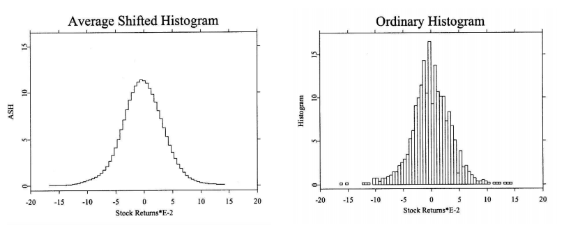
Averaged shifted histogram
Obtained by averaging over histograms with different bin origins. It has better convergence to $f(x)$than histograms and similar computational cost. It was introduced by Chamayou (1980) for the analysis of HEP data.
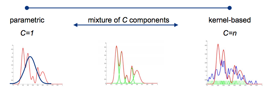
Mixture models
It is a semiparametric density estimation, a compact density estimation is created by combining $C$ parametric components (e.g. Gaussians). In the limit $C\rightarrow\infty$ it is a universal approximator and therefore a fully non-parametric method.
Resort to numerical procedures for fitting, most used algoritm is Expectation-Maximization (EM). In a way, they are a hybrid between parametric and Kernel methods.
Adaptative kernel density estimation
Variable/adaptative kernel estimation is based on modifying the kernel size based on the location of the samples $\{x_i\}$ and/or the location of the test point $f(x)$.
Some versions of this type of density estimators can be though of mixture of nearest neighbors and kernel density because the kernel size depend on the local density. They typically outperform fixed kernel kernel density in multi-dimensional problems (see article above).
Conclusions
There are many problems the underlying probability density function $f(x)$ is not known or cannot be expressed parametricaly. Non-parametric density estimation methods try to providing an estimation for $f(x)$ with as few assumptions as possible.
While histograms are asiduosly used for density estimation, they are biased estimators of $f(x)$ given their piecewise nature, specially in the oversmoothing regime. In addition they are no smooth and do not scale well in n-D problems.
Alternatives to histogram do exist, as the k nearest neighbor (kNN) estimator and the kernel density estimator (KDE), which typically provide better convergence at some additional computational cost.
When dealing with bias-variance trade-off on non-parametric density estimation, not bad idea to go for undersmoothing (more variance) because is easier to estimate based on the data direcly.
The use of advanced non-parametric methods (i.e. not histograms) in high energy physics is not very popular but they might be useful in several use cases.